参考
睿智的目标检测56——Pytorch搭建YoloV5目标检测平台
原理
前处理
网络结构
整体思想
思想框架
特征提取-特征加强-预测先验框对应的物体情况。
改进部分
1、主干部分:使用了Focus网络结构,具体操作是在一张图片中每隔一个像素拿到一个值,这个时候获得了四个独立的特征层,然后将四个独立的特征层进行堆叠,此时宽高信息就集中到了通道信息,输入通道扩充了四倍。该结构在yolov5第5版之前有所应用,最新版本中未使用。
2、数据增强:Mosaic数据增强、Mosaic利用了四张图片进行拼接实现数据中增强,根据论文所说其拥有一个巨大的优点是丰富检测物体的背景!且在BN计算的时候一下子会计算四张图片的数据!
3、多正样本匹配:在之前的Yolo系列里面,在训练时每一个真实框对应一个正样本,即在训练时,每一个真实框仅由一个先验框负责预测。YoloV5中为了加快模型的训练效率,增加了正样本的数量,在训练时,每一个真实框可以由多个先验框负责预测。
具体结构
对比参考1中的源码看,效果更佳。这里的输入输出以yolov5-l为例。v5有四种体量,分别为s,m,l,x,区别在于他们中间的维度以及CSP模块的叠加深度,width表示维度例如经过颈部结构输出分别为32,40,64,80;depth为CSP模块的叠加层数,第二个虚线框的叠加层数分别为1,2,3,4。
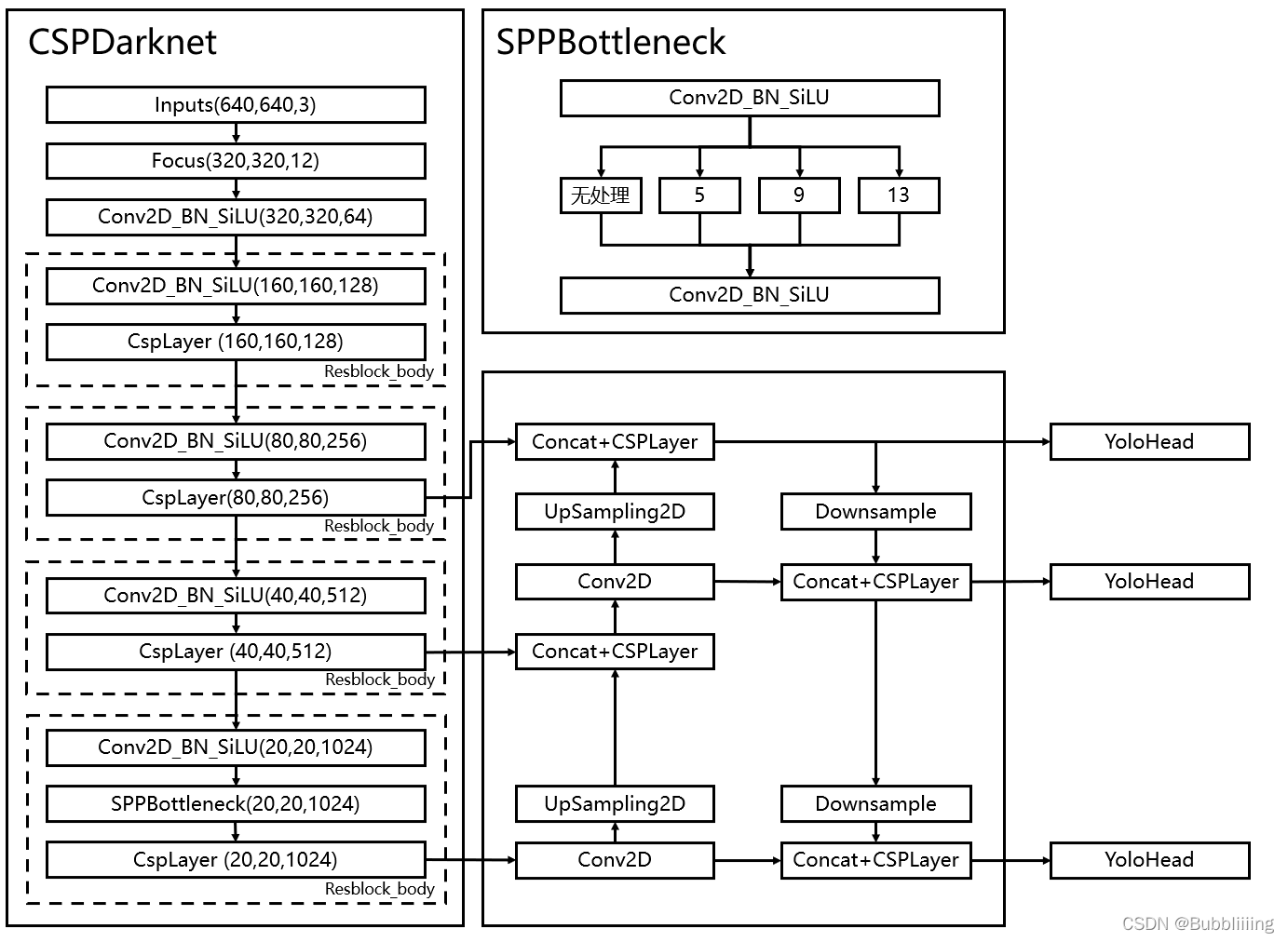
Backbone
(640, 640, 3)-->(80,80,256), (40,40,512), (20,20,1024)
1.颈部结构
(640, 640, 3)-->(320, 320, 12)-->(320, 320, 64)
(1)说明
yolo v5最初使用了Focus结构来初步提取特征,在改进后使用了大卷积核的卷积来初步提取特征。
(2)内部执行细节
class Focus(nn.Module):
    def __init__(self, c1, c2, k=1, s=1, p=None, g=1, act=True):
        super(Focus, self).__init__()
        # 这里的Conv表示卷积,归一化,激活函数三件套
        self.conv = Conv(c1 * 4, c2, k, s, p, g, act)

    def forward(self, x):
        # (320, 320, 12) => (320, 320, 64)
        return self.conv(
            # (640, 640, 3) => (320, 320, 12)
            torch.cat(
                [
                    x[..., ::2, ::2],
                    x[..., 1::2, ::2],
                    x[..., ::2, 1::2],
                    x[..., 1::2, 1::2]
                ], 1
            )
        )
(3)具体模块
Focus结构 + 1*1卷积

2.CSP模块
(320, 320, 64)-->(160, 160, 128)-->(160, 160, 128)
(160, 160, 128)-->(80, 80, 256)-->(80, 80, 256)
(80, 80, 256)-->(40, 40, 512)-->(40, 40, 512)
(1)说明
(2)内部执行细节
class C3(nn.Module):
    def __init__(self, c1, c2, n=1, shortcut=True, g=1, e=0.5):
        super(C3, self).__init__()
        # hidden_channel 中间维度的深度为输入的一半,减少参数
        c_ = int(c2 * e)
        self.cv1 = Conv(c1, c_, 1, 1)
        self.cv2 = Conv(c1, c_, 1, 1)
        self.cv3 = Conv(2 * c_, c2, 1)
        self.m = nn.Sequential(*[Bottleneck(c_, c_, shortcut, g, e=1.0) for _ in range(n)])
        # self.m = nn.Sequential(*[CrossConv(c_, c_, 3, 1, g, 1.0, shortcut) for _ in range(n)])

    def forward(self, x):
        # 将一个Bottleneck处理的张量和原始的张量cat到一起
        # (320, 320, 128)-->(320, 320, 128)
        return self.cv3(torch.cat(
            (
                # (320, 320, 128)-->(320, 320, 64)-->(320, 320, 64)-->(320, 320, 64)--(320, 320, 64)
                self.m(self.cv1(x)),
                # (320, 320, 128)-->(320, 320, 64)
                self.cv2(x)
            )
            , dim=1))
class Bottleneck(nn.Module):
# Standard bottleneck
def __init__(self, c1, c2, shortcut=True, g=1, e=0.5):
super(Bottleneck, self).__init__()
# hidden channels
c_ = int(c2 * e)
self.cv1 = Conv(c1, c_, 1, 1)
self.cv2 = Conv(c_, c2, 3, 1, g=g)
self.add = shortcut and c1 == c2
def forward(self, x):
return x + self.cv2(self.cv1(x)) if self.add else self.cv2(self.cv1(x))(3)具体模块
1)步长为2的3*3卷积块
2)CSP模块:Bottleneck内部是1个步长1的1*1和1个步长1的3*3卷积,并且设置了残差连接。注意这里的3*3卷积用了padding,保持输入输出一致。第三,四个虚线框除了降采样,还有的与第二个虚线框不一样的操作是CSP叠加的模块增加,第三,四个框增加第二个框的三倍。第五个框则与第二框深度一致,并且取消残差连接。
3.SPP模块
(40, 40, 512)-->(20, 20, 1024)-->(20, 20, 1024)-->(20, 20, 1024)
(1)说明
SPP原理及实现
Spatial Pyramid Pooling in Deep Convolutional Networks for Visual Recognition
SPP的代码如下,每步已显示变量结果,本质是将图像通过不同尺度的池化下采样再进入全连接层。
# coding=utf-8

import math
import torch
import torch.nn.functional as F


# 构建SPP层(空间金字塔池化层)
class SPPLayer(torch.nn.Module):

    def __init__(self, num_levels = 3, pool_type='max_pool'):
        super(SPPLayer, self).__init__()
        # 划分成多少份
        self.num_levels = num_levels
        # 池化的类型
        self.pool_type = pool_type

    def forward(self, x):
        # (16, 3, 256, 156)
        num, c, h, w = x.size()

        for i in range(self.num_levels):
            # level = 1, 2, 3
            level = i + 1
            # math.ceil返回不小于x的最接近的整数,kernel_size = (256, 256), (128, 128), (86, 86),stride = (256, 256), (128, 128), (86, 86)
            kernel_size = (math.ceil(h / level), math.ceil(w / level))
            stride = (math.ceil(h / level), math.ceil(w / level))
            # math向下取整,pooling用来填充用的,此处是(0, 0), (0, 0), (0, 0)
            pooling = (
            math.floor((kernel_size[0] * level - h + 1) / 2), math.floor((kernel_size[1] * level - w + 1) / 2))

            # 选择池化方式
            if self.pool_type == 'max_pool':
                # tensor = [16, 3], [16, 12], [16, 27]
                tensor = F.max_pool2d(x, kernel_size=kernel_size, stride=stride, padding=pooling).view(num, -1)
            else:
                tensor = F.avg_pool2d(x, kernel_size=kernel_size, stride=stride, padding=pooling).view(num, -1)

            # 把所有的张量cat到一起,格式:[batch, channel],[16, 3 + 12 + 27]
            if (i == 0):
                x_flatten = tensor.view(num, -1)
            else:
                x_flatten = torch.cat((x_flatten, tensor.view(num, -1)), 1)
        return x_flatten
x = torch.rand((16, 3, 256, 256))
SPPLayer().forward(x)
【YOLOv5】SPP、SPPF模块及添加ASPP模块
yolo v4中,SPP是用在FPN里面的,在yolo v5中,SPP模块被用在了主干特征提取网络中, 和yolo v3一样。yolo v5借鉴SPP的思想,即采用统一步长但不同尺寸的卷积核和补丁实现SPP。再通过concate按通道拼接后用1x1卷积,实现特征融合。
(2)内部执行细节
class SPP(nn.Module):
    def __init__(self, c1, c2, k=(5, 9, 13)):
        super(SPP, self).__init__()
        c_ = c1 // 2
        self.cv1 = Conv(c1, c_, 1, 1)
        self.cv2 = Conv(c_ * (len(k) + 1), c2, 1, 1)
        self.m = nn.ModuleList([nn.MaxPool2d(kernel_size=x, stride=1, padding=x // 2) for x in k])

    def forward(self, x):
        # (20, 20, 1024)-->(20, 20, 1024)
        x = self.cv1(x)
        # (20, 20, 1024), (20, 20, 1024), (20, 20, 1024), (20, 20, 1024)-->((20, 20, 1024))
        return self.cv2(torch.cat([x] + [m(x) for m in self.m], 1))
(3)具体模块
1)步长为2的3*3卷积块
2)SPP模块:与CSP的区别在于CSP主要是增加深度,SPP为增加宽度。这里借鉴SPP的思想,并没有搞入后面的全连接层。
3)CSP模块
总结:本质是1*1卷积,3*3卷积与残差连接的递进组合,1*1卷积负责维度对齐,3*3卷积多用于降采样。同时,借鉴CSP的维度加深策略,SPP特征加宽策略。
FPN + Yolo Head
(80,80,256), (40,40,512), (20,20,1024)-->(80,80,255), (40,40,255), (20,20,255)
(1)说明
255分别代表3 * (4 + 1 + num_classes),3代表3个先验框,4代表中心点坐标和宽高,1代表是否有物体,num_classes代表置信度。
(2)内部执行细节
# 步长为1的1*1卷积 20, 20, 1024 -> 20, 20, 512
        P5          = self.conv_for_feat3(feat3)
        # 最邻近上采样2倍大小 20, 20, 512 -> 40, 40, 512
        P5_upsample = self.upsample(P5)
        # cat 40, 40, 512 -> 40, 40, 1024
        P4          = torch.cat([P5_upsample, feat2], 1)
        # 叠加depth为第二个虚线框的CSP模块,且维度减半了 40, 40, 1024 -> 40, 40, 512
        P4          = self.conv3_for_upsample1(P4)

        # feat2,feat1和feat3,feat2执行相同的操作
        # 40, 40, 512 -> 40, 40, 256
        P4          = self.conv_for_feat2(P4)
        # 40, 40, 256 -> 80, 80, 256
        P4_upsample = self.upsample(P4)
        # 80, 80, 256 cat 80, 80, 256 -> 80, 80, 512
        P3          = torch.cat([P4_upsample, feat1], 1)
        # 80, 80, 512 -> 80, 80, 256
        P3          = self.conv3_for_upsample2(P3)

        # 步长为2的3*3卷积 80, 80, 256 -> 40, 40, 256
        P3_downsample = self.down_sample1(P3)
        # 40, 40, 256 cat 40, 40, 256 -> 40, 40, 512
        P4 = torch.cat([P3_downsample, P4], 1)
        # 叠加depth为第二个虚线框的CSP模块,维度不减半 40, 40, 512 -> 40, 40, 512
        P4 = self.conv3_for_downsample1(P4)

        # P4,P5执行相同的操作
        # 40, 40, 512 -> 20, 20, 512
        P4_downsample = self.down_sample2(P4)
        # 20, 20, 512 cat 20, 20, 512 -> 20, 20, 1024
        P5 = torch.cat([P4_downsample, P5], 1)
        # 20, 20, 1024 -> 20, 20, 1024
        P5 = self.conv3_for_downsample2(P5)

        # 以下均为1*1卷积,将得到的特征维数映射到回归层和类别层
        # 80, 80, 256 => 80, 80, 3 * (5 + num_classes) => 80, 80, 3 * (4 + 1 + num_classes)
        # 40, 40, 512 => 40, 40, 3 * (5 + num_classes) => 40, 40, 3 * (4 + 1 + num_classes)
        # 20, 20, 1024 => 20, 20, 3 * (5 + num_classes) => 20, 20, 3 * (4 + 1 + num_classes)
        #---------------------------------------------------#
        #   第三个特征层
        #   y3=(batch_size,255,80,80)
        #---------------------------------------------------#
        out2 = self.yolo_head_P3(P3)
        #---------------------------------------------------#
        #   第二个特征层
        #   y2=(batch_size,255,40,40)
        #---------------------------------------------------#
        out1 = self.yolo_head_P4(P4)
        #---------------------------------------------------#
        #   第一个特征层
        #   y1=(batch_size,255,20,20)
        #---------------------------------------------------#
        out0 = self.yolo_head_P5(P5)
(3)具体模块
后处理
(80,80,255), (40,40,255), (20,20,255)-->(25200, 85)-->((num_box_filter, 7))
预测框与得分
(80,80,255), (40,40,255), (20,20,255)-->( 3, 80, 80, 4), ( 3, 40, 40, 4), ( 3, 20, 20, 4);( 3, 80, 80, 1), ( 3, 40, 40, 1), ( 3, 20, 20, 1);( 3, 80, 80, 80), ( 3, 40, 40, 80), ( 3, 20, 20, 80)-->(19200, 85), (4800, 85), (1200, 85)-->(25200, 85)
(1)说明
yolo准备了9个不同大小的预测框10,13, 16,30, 33,23, 30,61, 62,45, 59,119, 116,90, 156,198, 373,326。前三个对应(20,20,255),中间三个对应(40,40,255),后三个对应(80,80,255)
(2)内部执行细节
1)将85中的5剖开分别进入激活函数
2)得到每个特征图的坐标位置和3个映射先验框,与x,y,w,h适配调节增大范围
a)进行中心预测点的计算,利用Regression预测结果前两个序号的内容对特征点的三个先验框中心坐标进行偏移。
b)进行预测框宽高的计算,利用Regression预测结果后两个序号的内容求指数后获得预测框的宽高。
3)归一化,聚合
        for i, input in enumerate(inputs):
            #-----------------------------------------------#
            #   输入的input一共有三个,他们的shape分别是
            #   batch_size = 1
            #   batch_size, 3 * (4 + 1 + 80), 20, 20
            #   batch_size, 255, 40, 40
            #   batch_size, 255, 80, 80
            #-----------------------------------------------#
            batch_size      = input.size(0)
            input_height    = input.size(2)
            input_width     = input.size(3)

            #-----------------------------------------------#
            #   输入为640x640时
            #   特征层相对于原图的变化 640/20, 640/40, 640/80
            #   stride_h = stride_w = 32、16、8
            #-----------------------------------------------#
            stride_h = self.input_shape[0] / input_height
            stride_w = self.input_shape[1] / input_width
            #-------------------------------------------------#
            #   此时获得的scaled_anchors大小是相对于特征层的
            #-------------------------------------------------#
            #   原图上的anchor映射到特征图上,这里求的是这个映射的尺度是多少
            scaled_anchors = [(anchor_width / stride_w, anchor_height / stride_h) for anchor_width, anchor_height in self.anchors[self.anchors_mask[i]]]

            #-----------------------------------------------#
            #   输入的input一共有三个,他们的shape分别是
            #   batch_size, 3, 20, 20, 85
            #   batch_size, 3, 40, 40, 85
            #   batch_size, 3, 80, 80, 85
            #-----------------------------------------------#
            #   将最后映射出来的张量做提前的格式转换,拿20*20的特征图举例(batch_size, 255, 20, 20)-->(batch_size, 3, 85, 20, 20)-->(batch_size, 3, 20, 20, 85)
            prediction = input.view(batch_size, len(self.anchors_mask[i]),
                                    self.bbox_attrs, input_height, input_width).permute(0, 1, 3, 4, 2).contiguous()

            #-----------------------------------------------#
            #   先验框的中心位置的调整参数
            #-----------------------------------------------#
            #   prediction[..., 0]为prediction前面所有维度保持不变,只把最后一维度切分
            #   (batch_size, 3, 20, 20, 85)-->(batch_size, 3, 20, 20)
            x = torch.sigmoid(prediction[..., 0])
            y = torch.sigmoid(prediction[..., 1])
            #-----------------------------------------------#
            #   先验框的宽高调整参数
            #-----------------------------------------------#
            w = torch.sigmoid(prediction[..., 2])
            h = torch.sigmoid(prediction[..., 3])
            #-----------------------------------------------#
            #   获得置信度,是否有物体
            #-----------------------------------------------#
            conf        = torch.sigmoid(prediction[..., 4])
            #-----------------------------------------------#
            #   种类置信度
            #-----------------------------------------------#
            pred_cls    = torch.sigmoid(prediction[..., 5:])

            FloatTensor = torch.cuda.FloatTensor if x.is_cuda else torch.FloatTensor
            LongTensor  = torch.cuda.LongTensor if x.is_cuda else torch.LongTensor

            #----------------------------------------------------------#
            #   生成网格,先验框中心,网格左上角
            #   batch_size,3,20,20
            #----------------------------------------------------------#
            # 得到间距为1的x,y[ 0.,  1.,  2.,  3.,  4.,  5.,  6.,  7.,  8.,  9., 10., 11., 12., 13., 14., 15., 16., 17., 18., 19.]-->
            # 在行上重复得到的shape为[20, 20]-->[batch_size*3, 20, 20]-->[batch_size, 3, 20, 20]
            grid_x = torch.linspace(0, input_width - 1, input_width).repeat(input_height, 1).repeat(
                batch_size * len(self.anchors_mask[i]), 1, 1).view(x.shape).type(FloatTensor)
            grid_y = torch.linspace(0, input_height - 1, input_height).repeat(input_width, 1).t().repeat(
                batch_size * len(self.anchors_mask[i]), 1, 1).view(y.shape).type(FloatTensor)

            #----------------------------------------------------------#
            #   按照网格格式生成先验框的宽高
            #   [batch_size,3,20,20]
            #----------------------------------------------------------#
            anchor_w = FloatTensor(scaled_anchors).index_select(1, LongTensor([0]))
            anchor_h = FloatTensor(scaled_anchors).index_select(1, LongTensor([1]))
            anchor_w = anchor_w.repeat(batch_size, 1).repeat(1, 1, input_height * input_width).view(w.shape)
            anchor_h = anchor_h.repeat(batch_size, 1).repeat(1, 1, input_height * input_width).view(h.shape)

            #----------------------------------------------------------#
            #   利用预测结果对先验框进行调整
            #   首先调整先验框的中心,从先验框中心向右下角偏移
            #   再调整先验框的宽高。
            #   x 0 ~ 1 => 0 ~ 2 => -0.5, 1.5 => 负责一定范围的目标的预测
            #   y 0 ~ 1 => 0 ~ 2 => -0.5, 1.5 => 负责一定范围的目标的预测
            #   w 0 ~ 1 => 0 ~ 2 => 0 ~ 4 => 先验框的宽高调节范围为0~4倍
            #   h 0 ~ 1 => 0 ~ 2 => 0 ~ 4 => 先验框的宽高调节范围为0~4倍
            #----------------------------------------------------------#
            pred_boxes          = FloatTensor(prediction[..., :4].shape)
            pred_boxes[..., 0]  = x.data * 2. - 0.5 + grid_x
            pred_boxes[..., 1]  = y.data * 2. - 0.5 + grid_y
            pred_boxes[..., 2]  = (w.data * 2) ** 2 * anchor_w
            pred_boxes[..., 3]  = (h.data * 2) ** 2 * anchor_h

            #----------------------------------------------------------#
            #   将输出结果归一化成小数的形式
            #----------------------------------------------------------#
            _scale = torch.Tensor([input_width, input_height, input_width, input_height]).type(FloatTensor)
            output = torch.cat((pred_boxes.view(batch_size, -1, 4) / _scale,
                                conf.view(batch_size, -1, 1), pred_cls.view(batch_size, -1, self.num_classes)), -1)
            outputs.append(output.data)
(3)具体模块
得分筛选与非极大值抑制
(25200, 85)-->(num_box, 85)-->(num_box, 7)(将那80转为类别和置信度)-->(num_box_filter, 7)
(1)说明
得分筛选就是筛选出得分满足confidence置信度的预测框。
非极大抑制就是筛选出一定区域内属于同一种类得分最大的框。
得分筛选-->得分过滤(85-->7)-->同一种类进行最大值抑制-->将得到的框的坐标值映射回原图
非极大值抑制:
1)是否有物体的置信度评分*该种类的置信度评分,降序排序
2)依次将现在的框与后面的框求IOU,利用IOU阈值筛选掉不满足阈值的情况
(2)内部执行细节
        for i, image_pred in enumerate(prediction):
            #----------------------------------------------------------#
            #   对种类预测部分取max。
            #   class_conf  [num_anchors, 1]    种类置信度
            #   class_pred  [num_anchors, 1]    种类
            #----------------------------------------------------------#
            class_conf, class_pred = torch.max(image_pred[:, 5:5 + num_classes], 1, keepdim=True)

            #----------------------------------------------------------#
            #   利用置信度进行第一轮筛选
            #----------------------------------------------------------#
            conf_mask = (image_pred[:, 4] * class_conf[:, 0] >= conf_thres).squeeze()

            #----------------------------------------------------------#
            #   根据置信度进行预测结果的筛选
            #----------------------------------------------------------#
            image_pred = image_pred[conf_mask]
            class_conf = class_conf[conf_mask]
            class_pred = class_pred[conf_mask]
            if not image_pred.size(0):
                continue
            #-------------------------------------------------------------------------#
            #   detections  [num_anchors, 7]
            #   7的内容为:x1, y1, x2, y2, obj_conf, class_conf, class_pred
            #-------------------------------------------------------------------------#
            detections = torch.cat((image_pred[:, :5], class_conf.float(), class_pred.float()), 1)

            #------------------------------------------#
            #   获得预测结果中包含的所有种类
            #------------------------------------------#
            unique_labels = detections[:, -1].cpu().unique()

            if prediction.is_cuda:
                unique_labels = unique_labels.cuda()
                detections = detections.cuda()

            for c in unique_labels:
                #------------------------------------------#
                #   获得某一类得分筛选后全部的预测结果
                #------------------------------------------#
                detections_class = detections[detections[:, -1] == c]

                #------------------------------------------#
                #   使用官方自带的非极大抑制会速度更快一些!
                #   筛选出一定区域内,属于同一种类得分最大的框
                #------------------------------------------#
                keep = nms(
                    detections_class[:, :4],
                    detections_class[:, 4] * detections_class[:, 5],
                    nms_thres
                )
                max_detections = detections_class[keep]

                # # 按照存在物体的置信度排序
                # _, conf_sort_index = torch.sort(detections_class[:, 4]*detections_class[:, 5], descending=True)
                # detections_class = detections_class[conf_sort_index]
                # # 进行非极大抑制
                # max_detections = []
                # while detections_class.size(0):
                #     # 取出这一类置信度最高的,一步一步往下判断,判断重合程度是否大于nms_thres,如果是则去除掉
                #     print(detections_class[0].unsqueeze(0).shape)
                #     max_detections.append(detections_class[0].unsqueeze(0))
                #     if len(detections_class) == 1:
                #         break
                #     ious = bbox_iou(max_detections[-1], detections_class[1:])
                #     detections_class = detections_class[1:][ious < nms_thres]
                # # 堆叠
                # max_detections = torch.cat(max_detections).data
                #
                # Add max detections to outputs
                output[i] = max_detections if output[i] is None else torch.cat((output[i], max_detections))

            if output[i] is not None:
                output[i]           = output[i].cpu().numpy()
                box_xy, box_wh      = (output[i][:, 0:2] + output[i][:, 2:4])/2, output[i][:, 2:4] - output[i][:, 0:2]
                output[i][:, :4]    = self.yolo_correct_boxes(box_xy, box_wh, input_shape, image_shape, letterbox_image)
(3)具体模块
损失函数(train)
(80,80,255), (40,40,255), (20,20,255)-->loss
(1)说明
1)损失函数用作训练,取Yolo Head之后的张量作为输入。
2)正样本匹配策略计算出适合这个真实框预测的先验框。
正样本匹配,就是寻找哪些先验框被认为有对应的真实框,并且负责这个真实框的预测。
a)宽高比匹配先验框
b)最邻近网格匹配特征点

3)包含三个部分的损失
a)Reg部分,IOU损失
b)Obj部分,所有真实框对应的先验框都是正样本,剩余的先验框均为负样本,根据正负样本和特征点的是否包含物体的预测结果计算交叉熵损失。
c)Cls部分,根据真实框的种类和先验框的种类预测结果计算交叉熵损失。
(2)内部执行细节
1)与后处理预测框与得分处理一致
2)计算IOU损失,有无样本的交叉熵损失,类别的交叉熵损失
    def forward(self, l, input, targets=None, y_true=None):
        #----------------------------------------------------#
        #   l               代表使用的是第几个有效特征层
        #   input的shape为  bs, 3*(5+num_classes), 20, 20
        #                   bs, 3*(5+num_classes), 40, 40
        #                   bs, 3*(5+num_classes), 80, 80
        #   targets         真实框的标签情况 [batch_size, num_gt, 5]
        #----------------------------------------------------#
        #--------------------------------#
        #   获得图片数量,特征层的高和宽
        #   20, 20
        #--------------------------------#
        bs      = input.size(0)
        in_h    = input.size(2)
        in_w    = input.size(3)
        #-----------------------------------------------------------------------#
        #   计算步长
        #   每一个特征点对应原来的图片上多少个像素点
        #   [640, 640] 高的步长为640 / 20 = 32,宽的步长为640 / 20 = 32
        #   如果特征层为20x20的话,一个特征点就对应原来的图片上的32个像素点
        #   如果特征层为40x40的话,一个特征点就对应原来的图片上的16个像素点
        #   如果特征层为80x80的话,一个特征点就对应原来的图片上的8个像素点
        #   stride_h = stride_w = 32、16、8
        #-----------------------------------------------------------------------#
        stride_h = self.input_shape[0] / in_h
        stride_w = self.input_shape[1] / in_w
        #-------------------------------------------------#
        #   此时获得的scaled_anchors大小是相对于特征层的
        #-------------------------------------------------#
        scaled_anchors  = [(a_w / stride_w, a_h / stride_h) for a_w, a_h in self.anchors]
        #-----------------------------------------------#
        #   输入的input一共有三个,他们的shape分别是
        #   bs, 3 * (5+num_classes), 20, 20 => bs, 3, 5 + num_classes, 20, 20 => batch_size, 3, 20, 20, 5 + num_classes

        #   batch_size, 3, 20, 20, 5 + num_classes
        #   batch_size, 3, 40, 40, 5 + num_classes
        #   batch_size, 3, 80, 80, 5 + num_classes
        #-----------------------------------------------#
        prediction = input.view(bs, len(self.anchors_mask[l]), self.bbox_attrs, in_h, in_w).permute(0, 1, 3, 4, 2).contiguous()

        #-----------------------------------------------#
        #   先验框的中心位置的调整参数
        #-----------------------------------------------#
        x = torch.sigmoid(prediction[..., 0])
        y = torch.sigmoid(prediction[..., 1])
        #-----------------------------------------------#
        #   先验框的宽高调整参数
        #-----------------------------------------------#
        w = torch.sigmoid(prediction[..., 2])
        h = torch.sigmoid(prediction[..., 3])
        #-----------------------------------------------#
        #   获得置信度,是否有物体
        #-----------------------------------------------#
        conf = torch.sigmoid(prediction[..., 4])
        #-----------------------------------------------#
        #   种类置信度
        #-----------------------------------------------#
        pred_cls = torch.sigmoid(prediction[..., 5:])
        #-----------------------------------------------#
        #   self.get_target已经合并到dataloader中
        #   原因是在这里执行过慢,会大大延长训练时间
        #-----------------------------------------------#
        # y_true, noobj_mask = self.get_target(l, targets, scaled_anchors, in_h, in_w)

        #---------------------------------------------------------------#
        #   将预测结果进行解码,判断预测结果和真实值的重合程度
        #   如果重合程度过大则忽略,因为这些特征点属于预测比较准确的特征点
        #   作为负样本不合适
        #----------------------------------------------------------------#
        pred_boxes = self.get_pred_boxes(l, x, y, h, w, targets, scaled_anchors, in_h, in_w)

        if self.cuda:
            y_true          = y_true.type_as(x)

        loss    = 0
        n       = torch.sum(y_true[..., 4] == 1)
        if n != 0:
            #---------------------------------------------------------------#
            #   计算预测结果和真实结果的giou,计算对应有真实框的先验框的giou损失
            #                         loss_cls计算对应有真实框的先验框的分类损失
            #----------------------------------------------------------------#
            giou        = self.box_giou(pred_boxes, y_true[..., :4]).type_as(x)
            loss_loc    = torch.mean((1 - giou)[y_true[..., 4] == 1])
            loss_cls    = torch.mean(self.BCELoss(pred_cls[y_true[..., 4] == 1], self.smooth_labels(y_true[..., 5:][y_true[..., 4] == 1], self.label_smoothing, self.num_classes)))
            loss        += loss_loc * self.box_ratio + loss_cls * self.cls_ratio
            #-----------------------------------------------------------#
            #   计算置信度的loss
            #   也就意味着先验框对应的预测框预测的更准确
            #   它才是用来预测这个物体的。
            #-----------------------------------------------------------#
            tobj        = torch.where(y_true[..., 4] == 1, giou.detach().clamp(0), torch.zeros_like(y_true[..., 4]))
        else:
            tobj        = torch.zeros_like(y_true[..., 4])
        loss_conf   = torch.mean(self.BCELoss(conf, tobj))

        loss        += loss_conf * self.balance[l] * self.obj_ratio
        # if n != 0:
        #     print(loss_loc * self.box_ratio, loss_cls * self.cls_ratio, loss_conf * self.balance[l] * self.obj_ratio)
        return loss
(3)具体模块